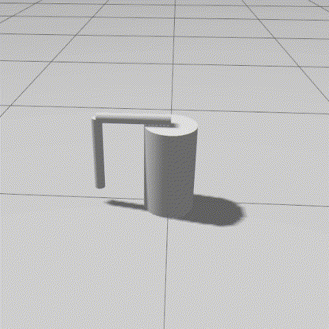
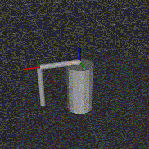
Furuta pendulum simulation
·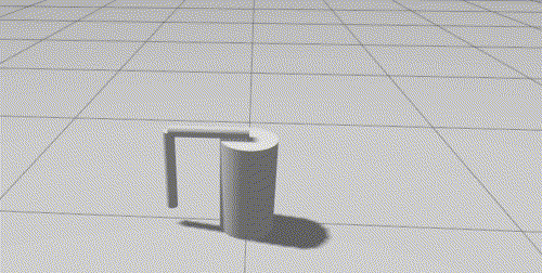
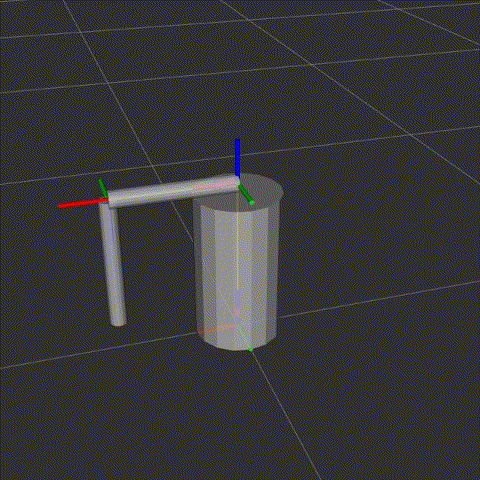
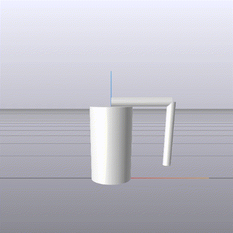
To refresh my knowledge about dynamical systems and to try out different control approaches in practice I decided to build a inverted pendulum. I chose a rotational variant mainly because I wanted to reuse it as a desktop toy, and it is more compact. While waiting for parts to arrive, I started playing around with different control approaches, and in this part I will summarize my adventures.
Classical approach
I will begin with something more classical, as it was taught in my uni courses. So first we derive differential equations that describe the dynamics of our system, linearize it around the upward position point and based on this design LQR controller. Here you can find a great resource that I used to get equations and linearized system. One slight simplification that I made was assuming torque control of the motor (so I didn’t model the motor’s equations and used torque as a control value). This assumption is also present in the other approaches.
After getting A and B matrices of the system, it was necessary to choose weights (Q and R). As I plan to use a slip ring to allow the pendulum to rotate freely, without limits, I put 0.0 weight on the first angle. Then I set the highest weight on the second angle, as it is the most important. For remaining velocities and control weights I put 1.0 (that was more of playing around, what worked best). Then to get K gains I used the control python library (all code is in the lqr.ipynb).
Now to verify the controller I implemented differential equations as the simulation node. The controller worked well when stabilizing the pendulum near the upward position, and responded properly to some disturbance torque (tau2 in equations), which is equal to pushing the pendulum. But, as this controller was based only on linearization around the upward position, it doesn’t work in other positions. So to get our pendulum upward from the initial downward position, we need something more - that is a swing-up. I used the approach described in Swing-up time analysis of pendulum namely Energy based swing-up control. Now our controller has two parts - in the initial downward position it uses swing-up and once the angle is close enough to the upward position it switches to the LQR.
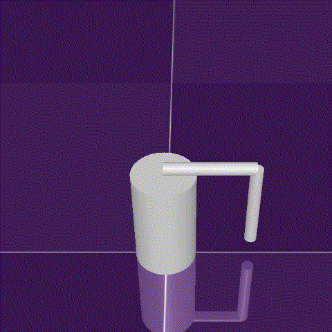
Using the same equations to design a controller and then validate it may not be the best option. To further verify it, I also created a simulation in Gazebo and surprisingly, it also worked there!
Drake
Well, derivation of motion equations and linearizing is quite a lot of hustle, maybe there is some way to omit it? Of course there is! Drake toolbox allows you to load a model from URDF and based on it, it can design an LQR controller automatically. Similarly to the previous approach, now it is only necessary to add a swing-up and once again we have a controller, but now faster! K gains achieved are quite close to previous ones:
| Classical approach | [-3.117e-15, 19.270, -1.000, 4.352] |
| Drake | [-2.922e-17, 18.931, -0.980, 4.265] |
Control toolbox
So now we have LQR with swing-up, which we created quite efficiently. But you know what is not yet efficient? Movement of the pendulum! We need something better, something optimal. And why not, this time we will use a different library. Control toolbox got you covered not only in terms of linearity, but also non-linear optimal control. But first, before creating a controller we have to import our pendulum. Once again, we won’t need hand-derived motion equations, we will use a model of the pendulum. Unfortunately, this time it won’t be that straightforward. First it is necessary to convert URDF to kindsl and drdsl files, then generate code using them. After finally getting our model to work, we can move on to designing the controller.
First I decided to calculate LQR once again, comparing gains, they are again quite close:
| Classical approach | [-3.117e-15, 19.270, -1.000, 4.352] |
| Drake | [-2.922e-17, 18.931, -0.980, 4.265] |
| Control Toolbox | [-6.869e-15, 19.182, -1.000, 4.356] |
After all these preparations we can move on to the MPC. As in the inverted pendulum example from the Control Toolbox iLQR was used, but the problem was additionally constrained on the control signal and both velocities. I chose a long time horizon (2.5s), which basically covers the whole motion of the pendulum from the downward to the upward position. It resulted in really efficient movement, but on the other hand, it requires substantial computing resources. Now look at this motion, it sure is more impressive!
Reinforcement Learning
Another control approach I decided to try was Deep Reinforcement Learning. I used Mujoco for simulation and Stable-Baselines3 for RL algorithms implementation.
As the full control problem, from the downward position to the upward stabilization, is quite complex, I decided to take smaller steps. I created 3 environments:
- Upward stabilization - the pendulum starts with an angle a little off the upward position, and with some small velocity (both values are drawn from the uniform distribution). The agent’s task is to keep the absolute value of the pendulum’s angle below a certain threshold. For every step it receives a reward, and if the angle is greater than some threshold, the episode is terminated. I was able to solve this problem with the PPO algorithm, the only thing I tuned was the number of total timesteps (length of training).
- Swing-up - this time pendulum starts in the downward position, and the agent’s task is getting the pendulum’s angle below a certain threshold (so that pendulum will be near the upward position). After getting below the threshold episode is terminated. This time as a reward I used the quadratic cost function (the same as is used in LQR, but with a minus) with weights that I used previously in LQR. Once again I was able to solve it with PPO, I only had to increase the number of timesteps.
- Full control problem - the pendulum starts in the downward position, the agent has to swing up and then also stabilize the pendulum. Basically, the only difference from the previous environment is that episode doesn’t terminate after the pendulum gets to the upward position. As a matter of fact, it doesn’t terminate until it reaches max episode length. The reward function is the same as in the previous step. This time solving the problem wasn’t as straightforward, I tried different algorithms (A2C, DDPG, PPO, SAC, TD3), mainly tuning the number of episodes and network architecture. I was able to achieve satisfactory results only with SAC, after increasing the size of the network to (512, 512, 512).
Verification
Every approach worked, but every single one used a different simulation. To better compare them and verify, it would be best to use a single simulator. I decided to use Gazebo and DE simulations - they already had ROS 2 interface and I also implemented every controller as a ROS 2 node.
In the Gazebo simulation every approach worked, but in case of the RL method difference is visible - the controller is much slower in getting to the upward position. The interesting thing is that it got the general idea of how to swing it up, and even with differences in the behavior of the pendulum, it was still able to achieve the goal.
In the simulation based on DEs, I found a problem with the MPC method, as it didn’t work at all. I tried tunning its parameters but still was unsuccessful. For now, the best explanation for this behavior I have is the differences between models, but it still seems quite strange, and I’m not really convinced about it. In the following weeks, I will try to debug it more.
Next steps
Now it is time to construct the pendulum! I hope that testing 3 different approaches across 5 simulations will result in at least one working solution.